Wind Speed Distributions and Fitting a Weibull Distribution

A wind speed distribution created using measured data is a good way to show the frequency of occurrence of different wind speeds for a particular location. Wind speed distribution can be used in conjunction wind a turbine power curve to estimate the potential electrical energy production for a specific wind turbine for a specific location.

The curve produced by a wind speed distribution can be approximated using a Weibull distribution. The following sections will describe how both a wind speed distribution taken from measured data as well as a fitted Weibull distribution are created using measured wind speed data.

Wind Speed Distribution taken from Measured Data

The figure below shows a measured wind speed data presented as a distribution (in blue) and a fitted Weibull distribution (in red):

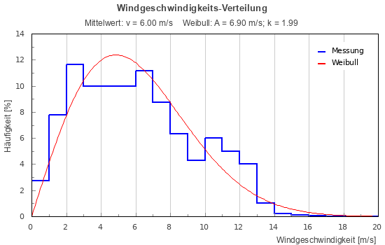
Making a wind speed distribution using measured data

In order to produce a wind speed distribution using measured data, wind speed ‘bins‘ are used to group and count the individual values for wind speed. For example, the first 3 wind speed bins in a wind distribution may be 0-1 m/s, 1-2 m/s and 2-3 m/s. Any wind speed values which fall within these ranges (bins) are grouped together and counted. By knowing the number of wind speed values within each bin as well as the total number of values for all wind speeds, it is possible to calculate the % frequency of the wind speeds associated with any of the wind speed bins. This process is carried out automatically by the WRE Web App and WRE v1.7.

The Weibull Distribution Curve

The following sections describe the Weibull distribution and explains calculation of Weibull distribution parameters (c and k) using the WAsP Method. The Weibull distribution is a continuous probability distribution with the following expression:

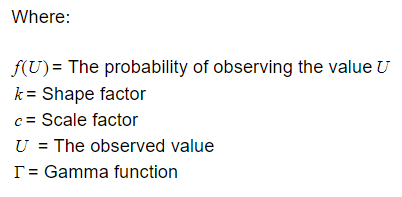
• The scale parameter, c, is the Weibull scale factor in m/s; a measure for the characteristic wind speed of the distribution.

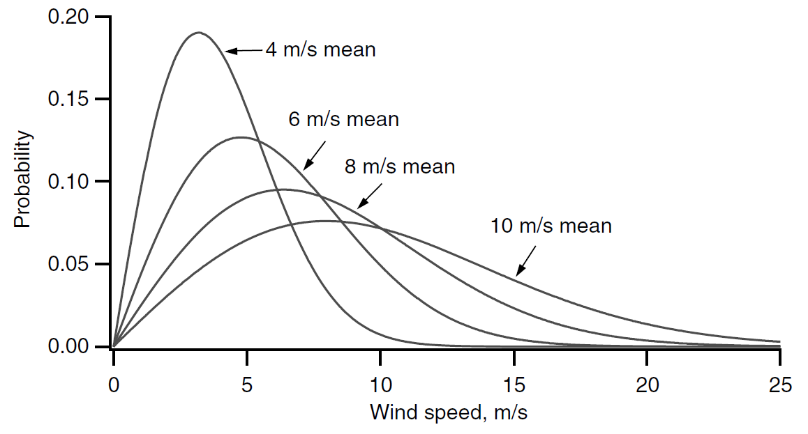
• The shape parameter, k. is the Weibull shape factor. It specifies the shape of a Weibull distribution and takes on a value of between 1 and 3. A small value for k signifies very variable winds, while constant winds are characterised by a larger k. Also, the higher the value of k, the higher the median wind speed.

To determine the scale and shape parameters, the following expressions need to be used: 1st Moment, Cumulative Function for the Weibull Distribution and the 3rd Moment. These are defined in the following sections.

1st Moment:

The 1st moment is denoted by <u>. It is equal to the mean of the sample. Or it can be calculated using the following formula:

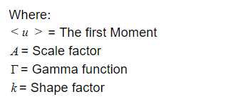
Tip: When using the observation data, we can calculate the mean and effectively assign a value to <u> in the above formula.

Cumulative Function for the Weibull Distribution:

3rd Moment:

The 3rd moment is denoted by <u3>. It is equal to:

• average of [(the difference between each observed value and the average)^3 ] . 
• Or it can be calculated using the following formula:

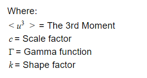
Finding c and k

By combining the Equations 2 and 4, an equation with only k unknown is obtained (Equation 5). Solving that equation with a zero-finding algorithm, or a goal seek within excel, will return k.

Next, c is calculated using Equation 2 and the value of k derived from Equation 4 .

Using c, k and U values to form a Weibull distribution

Now that c and k have been derived from the observational data, different U values can be substituted into the Equation 1, which is the Weibull distribution function: